December 03, 2020

Sébastien Labbé

Tiling a polyomino with polyominoes in SageMath

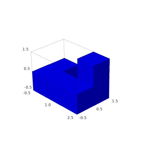
Suppose that you 3D print many copies of the following 3D hexo-mino at home:

sage: from sage.combinat.tiling import Polyomino, TilingSolver
sage: p = Polyomino([(0,0,0), (0,1,0), (1,0,0), (2,0,0), (2,1,0), (2,1,1)], color='blue')
sage: p.show3d()
Launched html viewer for Graphics3d Object
/Files/2020/polyomino.png

You would like to know if you can tile a larger polyomino or in particular a rectangular box with many copies of it. The TilingSolver module in SageMath is made for that. See also this recent question on ask.sagemath.org.

sage: T = TilingSolver([p], (7,5,3), rotation=True, reflection=False, reusable=True)
sage: T
Tiling solver of 1 pieces into a box of size 24
Rotation allowed: True
Reflection allowed: False
Reusing pieces allowed: True

There is no solution when tiling a box of shape 7x5x3 with this polyomino:

sage: T.number_of_solutions()
0

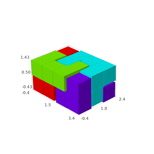
But there are 4 solutions when tiling a box of shape 4x3x2 with this polyomino:

sage: T = TilingSolver([p], (4,3,2), rotation=True, reflection=False, reusable=True)
sage: T.number_of_solutions()
4

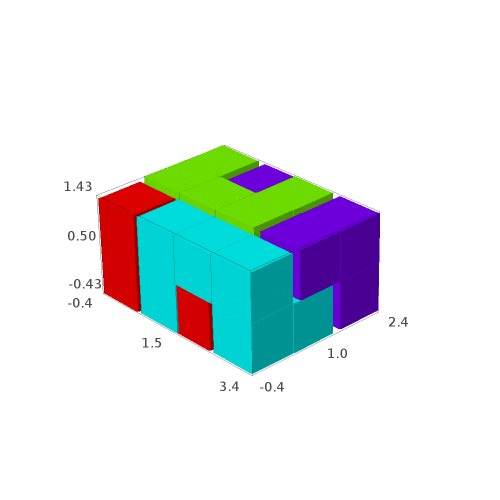
We construct the list of solutions:

sage: solutions = [sol for sol in T.solve()]

Each solution contains the isometric copies of the polyominoes tiling the box:

sage: solutions[0]
[Polyomino: [(0, 0, 0), (0, 0, 1), (0, 1, 0), (1, 1, 0), (2, 0, 0), (2, 1, 0)], Color: #ff0000,
 Polyomino: [(0, 1, 1), (0, 2, 0), (0, 2, 1), (1, 1, 1), (2, 1, 1), (2, 2, 1)], Color: #ff0000,
 Polyomino: [(1, 0, 0), (1, 0, 1), (2, 0, 1), (3, 0, 0), (3, 0, 1), (3, 1, 0)], Color: #ff0000,
 Polyomino: [(1, 2, 0), (1, 2, 1), (2, 2, 0), (3, 1, 1), (3, 2, 0), (3, 2, 1)], Color: #ff0000]

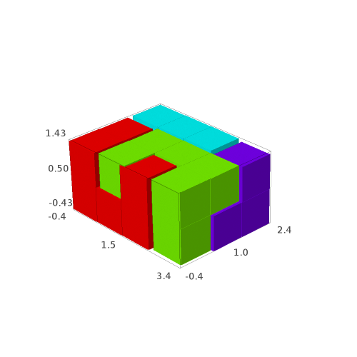
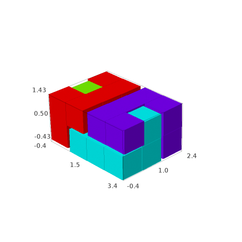
It may be easier to visualize the solutions, so we define the following function allowing to draw the solutions with different colors for each piece:

sage: def draw_solution(solution, size=0.9):
....:     colors = rainbow(len(solution))
....:     for piece,col in zip(solution, colors):
....:         piece.color(col)
....:     return sum((piece.show3d(size=size) for piece in solution), Graphics())
sage: G = [draw_solution(sol) for sol in solutions]
sage: G
[Graphics3d Object, Graphics3d Object, Graphics3d Object, Graphics3d Object]
sage: G[0]   # in Sage, this will open a 3d viewer automatically
/Files/2020/solution0.png
sage: G[1]
/Files/2020/solution1.png
sage: G[2]
/Files/2020/solution2.png
sage: G[3]
/Files/2020/solution3.png

We may save the solutions to a file:

sage: G[0].save('solution0.png', aspect_ratio=1, zoom=1.2)
sage: G[1].save('solution1.png', aspect_ratio=1, zoom=1.2)
sage: G[2].save('solution2.png', aspect_ratio=1, zoom=1.2)
sage: G[3].save('solution3.png', aspect_ratio=1, zoom=1.2)

Question: are all of the 4 solutions isometric to each other?

The tiling problem is solved due to a reduction to the exact cover problem for which dancing links Knuth's algorithm provides all the solutions. One can see the rows of the dancing links matrix as follows:

sage: d = T.dlx_solver()
sage: d
Dancing links solver for 24 columns and 56 rows
sage: d.rows()
[[0, 1, 2, 4, 5, 11],
 [6, 7, 8, 10, 11, 17],
 [12, 13, 14, 16, 17, 23],
 ...
 [4, 6, 7, 9, 10, 11],
 [10, 12, 13, 15, 16, 17],
 [16, 18, 19, 21, 22, 23]]

The solutions to the dlx solver can be obtained as follows:

sage: it = d.solutions_iterator()
sage: next(it)
[3, 36, 19, 52]

These are the indices of the rows each corresponding to an isometric copy of the polyomino within the box.

Since SageMath-9.2, the possibility to reduce the problem to a MILP problem or a SAT instance was added to SageMath (see #29338 and #29955):

sage: d.to_milp()
(Boolean Program (no objective, 56 variables, 24 constraints),
 MIPVariable of dimension 1)
sage: d.to_sat_solver()
CryptoMiniSat solver: 56 variables, 2348 clauses.

by Sébastien Labbé at December 03, 2020 01:48 PM

April 13, 2020

William Stein

DataDog: Don't make the same mistake I did -- a followup and thoughts about very unhappy customers

This is a followup to my previous blog post about DataDog billing.

TL;DR:
- I don't recommend DataDog,
- dealing with unhappy customers is hard,
- monitoring for data science nerds?

Hacker News Comments

DataDog at Google Cloud Summit

I was recently at the Seattle Google Cloud Summit and DataDog was well represented, with the biggest booth and top vendor billing during the keynote. Clearly they are doing something right. I had a past unpleasant experience with them, and I had just been auditing my records and discovered that last year DataDog had actually charged me a lot more than I thought, so was kind of annoyed. Nonetheless, they kept coming up and talking to me, server monitoring is life-and-death important to me, and their actual software is very impressive in some ways.

Nick Parisi started talking with me about DataDog. He sincerely wanted to know about my past experience with monitoring and the DataDog product, which he was clearly very enthuisiastic about. So I told him a bit, and he encouraged me to tell him more, explaining that he did not work at DataDog last year, and that he would like to know what happened. So he gave me his email, and he was very genuinely concerned and helpful, so I sent him an email with a link to my post, etc. I didn't receive a response, so a week later I asked why, and received a followup email from Jay Robichau, who is DataDog's Director of Sales.

Conference Call with DataDog

Jay setup a conference call with me today at 10am (September 22, 2017). Before the call, I sent him a summary of my blog post, and also requested a refund, especially for the suprise bill they sent me nearly 6 weeks after my post.

During the call, Jay explained that he was "protecting" Nick from me, and that I would mostly talk with Michelle Danis who is in charge of customer success. My expectation for the call is that we would find some common ground, and that they would at least appreciate the chance to make things right and talk with an unhappy customer. I was also curious about how a successful startup company addresses the concerns of an unhappy customer (me).

I expected the conversation to be difficult but go well, with me writing a post singing the praises of the charming DataDog sales and customer success people. A few weeks ago CoCalc.com (my employer) had a very unhappy customer who got (rightfully) angry over a miscommunication, told us he would no longer use our product, and would definitely not recommend it to anybody else. I wrote to him wanting to at least continue the discussion and help, but he was completely gone. I would do absolutely anything I could to ensure he is a satisfied, if only he would give me the chance. Also, there was a recent blog post from somebody unhappy with using CoCalc/Sage for graphics, and I reached out to them as best I could to at least clarify things...

In any case, here's what DataDog charged us as a result of us running their daemon on a few dozen containers in our Kubernetes cluster (a contractor who is not a native English speaker actually setup these monitors for us):

07/22/2016  449215JWJH87S8N4  DATADOG 866-329-4466 NY  $639.19
08/29/2016 2449215L2JH87V8WZ DATADOG 866-329-4466 NY $927.22

I was shocked by the 07/22 bill which spured my post, and discovered the 8/29 one only later. We canceled our subscription on July 22 (cancelling was difficult in itself).

Michelle started the conference call by explaining that the 08/29 bill was for charges incurred before 07/22, and that their billing system has over a month lag (and it does even today, unlike Google Cloud Platform, say). Then Michelle explained at length many of the changes that DataDog has made to their software to address the issues I (and others?) have pointed out with their pricing description and billing. She was very interested in whether I would be a DataDog customer in the future, and when I said no, she explained that they would not refund my money since the bill was not a mistake.

I asked if they now provide a periodic summary of the upcoming bill, as Google cloud platform (say) does. She said that today they don't, though they are working on it. They do now provide a summary of usage so far in an admin page.

Finally, I explained in no uncertain terms that I felt misled by their pricing. I expected that they would understand, and pointed out that they had just described to me many ways in which they were addressing this very problem. Very surprisingly, Michelle's response was that she absolutely would not agree that there was any problem with their pricing description a year ago, and they definitely would not refund my money. She kept bringing up the terms of service. I agreed that I didn't think legally they were in the wrong, given what she had explained, just that -- as they had just pointed out -- their pricing and billing was unclear in various ways. They would not agree at all.

I can't recommend doing business with DataDog. I had very much hoped to write the opposite in this updated post. Unfortunately, their pricing and terms are still confusing today compared to competitors, and they are unforgiving of mistakes. This dog bites.    

(Disclaimer: I took notes during the call, but most of the above is from memory, and I probably misheard or misunderstood something. I invite comments from DataDog to set the record straight.)

Also, for what it is worth, I definitely do recommend Google Cloud Platform.  They put in the effort to do many things right regarding clear billing.

How do Startups Deal with Unhappy Customers?

I am very curious about how other startups deal with unhappy customers. At CoCalc we have had very few "major incidents" yet... but I want to be as prepared as possible. At the Google Cloud Summit, I went to some amazing "war storries by SRE's" session in which they talked about situations they had been in years ago in which their decisions meant the difference between whether they would have a company or job tomorrow or not. These guys clearly have amazing instincts for when a problem was do-or-die serious and when it wasn't. And their deep preparation "in depth" was WHY they were on that stage, and a big reason why older companies like Google are still around. Having a strategy for addressing very angry customers is surely just as important.


Google SRE's: these guys are serious.

I mentioned my DataDog story to a long-time Google employee there (16 years!) and he said he had recently been involved in a similar situation with Google's Stackdriver monitoring, where the bill to a customer was $85K in a month just for Stackdriver. I asked what Google did, and he said they refunded the money, then worked with the customer to better use their tools.

There is of course no way to please all of the people all of the time. However, I genuinely feel that I was ripped off and misled by DataDog, but I have the impression that Jay and Michelle honestly view me as some jerk trying to rip them off for $1500.   And they probably hate me for telling you about my experiences.

So far, with CoCalc we charge customers in advance for any service we provide, so less people are surprised by a bill.  Sometimes there are problems with recurring subscriptions when a person is charged for the upcoming month of a subscription, and don't want to continue (e.g., because their course is over), we always fully refund the charge. What does your company do? Why? I do worry that our billing model means that we miss out on potential revenue.

We all know what successful huge consumer companies like Amazon and Wal-Mart do.

Monitoring for Data Science Nerds?

I wonder if there is interest in a service like DataDog, but targeted at Data Science Nerds, built on CoCalc, which provides hosted collaborative Jupyter notebooks with Pandas, R, etc., pre-installed. This talk at PrometheusCon 2017 mostly discussed the friction that people face moving data from Prometheus to analyze using data science tools (e.g., R, Python, Jupyter). CoCalc provides a collaborative data science environment, so if we were to smooth over those points of friction, perhaps it could be useful to certain people. And much more efficient...


---


by William Stein ([email protected]) at April 13, 2020 01:38 PM

March 27, 2020

Sébastien Labbé

Computer experiments for the Lyapunov exponent for MCF algorithms when dimension is larger than 3

In November 2015, I wanted to share intuitions I developped on the behavior of various distinct Multidimensional Continued Fractions algorithms obtained from various kind of experiments performed with them often involving combinatorics and digitial geometry but also including the computation of their first two Lyapunov exponents.

As continued fractions are deeply related to the combinatorics of Sturmian sequences which can be seen as the digitalization of a straight line in the grid \(\mathbb{Z}^2\), the multidimensional continued fractions algorithm are related to the digitalization of a straight line and hyperplanes in \(\mathbb{Z}^d\).

This is why I shared those experiments in what I called 3-dimensional Continued Fraction Algorithms Cheat Sheets because of its format inspired from typical cheat sheets found on the web. All of the experiments can be reproduced using the optional SageMath package slabbe where I share my research code. People asked me whether I was going to try to publish those Cheat Sheets, but I was afraid the format would change the organization of the information and data in each page, so, in the end, I never submitted those Cheat Sheets anywhere.

Here I should say that \(d\) stands for the dimension of the vector space on which the involved matrices act and \(d-1\) is the dimension of the projective space on which the algorithm acts.

One of the consequence of the Cheat Sheets is that it made us realize that the algorithm proposed by Julien Cassaigne had the same first two Lyapunov exponents as the Selmer algorithm (first 3 significant digits were the same). Julien then discovered the explanation as its algorithm is conjugated to some semi-sorted version of the Selmer algorihm. This result was shared during WORDS 2017 conference. Julien Leroy, Julien Cassaigne and I are still working on the extended version of the paper. It is taking longer mainly because of my fault because I have been working hard on aperiodic Wang tilings in the previous 2 years.

During July 2019, Wolfgang, Valérie and Jörg asked me to perform computations of the first two Lyapunov exponents for \(d\)-dimensional Multidimensional Continued Fraction algorithms for \(d\) larger than 3. The main question of interest is whether the second Lyapunov exponent keeps being negative as the dimension increases. This property is related to the notion of strong convergence almost everywhere of the simultaneous diopantine approximations provided by the algorithm of a fixed vector of real numbers. It did not take me too long to update my package since I had started to generalize my code to larger dimensions during Fall 2017. It turns out that, as the dimension increases, all known MCF algorithms have their second Lyapunov exponent become positive. My computations were thus confirming what they eventually published in their preprint in November 2019.

My motivation for sharing the results is the conference Multidimensional Continued Fractions and Euclidean Dynamics held this week (supposed to be held in Lorentz Center, March 23-27 2020, it got cancelled because of the corona virus) where some discussions during video meetings are related to this subject.

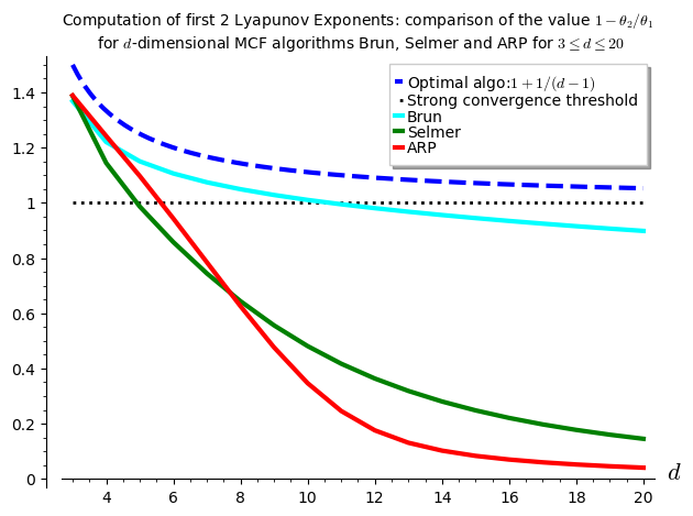
The computations performed below can be summarized in one graphics showing the values of \(1-\theta_2/\theta_1\) with respect to \(d\) for various \(d\)-dimensional MCF algorithms. It seems that \(\theta_2\) is negative up to dimension 10 for Brun, up to dimension 4 for Selmer and up to dimension 5 for ARP.

/Files/2020/lyapunov_exponent_comparison.png

I have to say that I was disapointed by the results because the algorithm Arnoux-Rauzy-Poincaré (ARP) that Valérie and I introduced was not performing so well as its second Lyapunov exponent seems to become positive for dimension \(d\geq 6\). I had good expectations for ARP because it reaches the highest value for \(1-\theta_2/\theta_1\) in the computations performed in the Cheat Sheets, thus better than Brun, better than Selmer when \(d=3\).

The algorithm for the computation of the first two Lyapunov exponents was provided to me by Vincent Delecroix. It applies the algorithm \((v,w)\mapsto(M^{-1}v,M^T w)\) millions of times. The evolution of the size of the vector \(v\) gives the first Lyapunov exponent. The evolution of the size of the vector \(w\) gives the second Lyapunov exponent. Since the computation is performed on 64-bits double floating point number, their are numerical issues to deal with. This is why some Gramm Shimdts operation is performed on the vector \(w\) at each time the vectors are renormalized to keep the vector \(w\) orthogonal to \(v\). Otherwise, the numerical errors cumulate and the computed value for the \(\theta_2\) becomes the same as \(\theta_1\). You can look at the algorithm online starting at line 1723 of the file mult_cont_frac_pyx.pyx from my optional package.

I do not know from where Vincent took that algorithm. So, I do not know how exact it is and whether there exits any proof of lower bounds and upper bounds on the computations being performed. What I can say is that it is quite reliable in the sense that is returns the same values over and over again (by that I mean 3 common most significant digits) with any fixed inputs (number of iterations).

Below, I show the code illustrating how to reproduce the results.

The version 0.6 (November 2019) of my package slabbe includes the necessary code to deal with some \(d\)-dimensional Multidimensional Continued Fraction (MCF) algorithms. Its documentation is available online. It is a PIP package, so it can be installed like this:

sage -pip install slabbe

Recall that the dimension \(d\) below is the linear one and \(d-1\) is the dimension of the space for the corresponding projective algorithm.

Import the Brun, Selmer and Arnoux-Rauzy-Poincaré MCF algorithms from the optional package:

sage: from slabbe.mult_cont_frac import Brun, Selmer, ARP

The computation of the first two Lyapunov exponents performed on one single orbit:

sage: Brun(dim=3).lyapunov_exponents(n_iterations=10^7)
(0.30473782969922547, -0.11220958022368056, 1.3682167728713919)

The starting point is taken randomly, but the results of the form of a 3-tuple \((\theta_1,\theta_2,1-\theta_2/\theta_1)\) are about the same:

sage: Brun(dim=3).lyapunov_exponents(n_iterations=10^7)
(0.30345018206132324, -0.11171509867725296, 1.3681497170915415)

Increasing the dimension \(d\) yields:

sage: Brun(dim=4).lyapunov_exponents(n_iterations=10^7)
(0.32639514522732005, -0.07191456560115839, 1.2203297648654456)
sage: Brun(dim=5).lyapunov_exponents(n_iterations=10^7)
(0.30918877340506756, -0.0463930802132972, 1.1500477514185734)

It performs an orbit of length \(10^7\) in about .5 seconds, of length \(10^8\) in about 5 seconds and of length \(10^9\) in about 50 seconds:

sage: %time Brun(dim=3).lyapunov_exponents(n_iterations=10^7)
CPU times: user 540 ms, sys: 0 ns, total: 540 ms
Wall time: 539 ms
(0.30488799356325225, -0.11234354880132114, 1.3684748208296182)
sage: %time Brun(dim=3).lyapunov_exponents(n_iterations=10^8)
CPU times: user 5.09 s, sys: 0 ns, total: 5.09 s
Wall time: 5.08 s
(0.30455473631148755, -0.11217550411862384, 1.3683262505689446)
sage: %time Brun(dim=3).lyapunov_exponents(n_iterations=10^9)
CPU times: user 51.2 s, sys: 0 ns, total: 51.2 s
Wall time: 51.2 s
(0.30438755982577026, -0.11211562816821799, 1.368331834035505)

Here, in what follows, I must admit that I needed to do a small fix to my package, so the code below will not work in version 0.6 of my package, I will update my package in the next days in order that the computations below can be reproduced:

sage: from slabbe.lyapunov import lyapunov_comparison_table

For each \(3\leq d\leq 20\), I compute 30 orbits and I show the most significant digits and the standard deviation of the 30 values computed.

For Brun algorithm:

sage: algos = [Brun(d) for d in range(3,21)]
sage: %time lyapunov_comparison_table(algos, n_orbits=30, n_iterations=10^7, ncpus=8)
CPU times: user 190 ms, sys: 2.8 s, total: 2.99 s
Wall time: 6min 31s
  Algorithm     \#Orbits   $\theta_1$ (std)     $\theta_2$ (std)      $1-\theta_2/\theta_1$ (std)
+-------------+----------+--------------------+---------------------+-----------------------------+
  Brun (d=3)    30         0.3045 (0.00040)     -0.1122 (0.00017)     1.3683 (0.00022)
  Brun (d=4)    30         0.32632 (0.000055)   -0.07188 (0.000051)   1.2203 (0.00014)
  Brun (d=5)    30         0.30919 (0.000032)   -0.04647 (0.000041)   1.1503 (0.00013)
  Brun (d=6)    30         0.28626 (0.000027)   -0.03043 (0.000035)   1.1063 (0.00012)
  Brun (d=7)    30         0.26441 (0.000024)   -0.01966 (0.000027)   1.0743 (0.00010)
  Brun (d=8)    30         0.24504 (0.000027)   -0.01207 (0.000024)   1.04926 (0.000096)
  Brun (d=9)    30         0.22824 (0.000021)   -0.00649 (0.000026)   1.0284 (0.00012)
  Brun (d=10)   30         0.2138 (0.00098)     -0.0022 (0.00015)     1.0104 (0.00074)
  Brun (d=11)   30         0.20085 (0.000015)   0.00106 (0.000022)    0.9947 (0.00011)
  Brun (d=12)   30         0.18962 (0.000017)   0.00368 (0.000021)    0.9806 (0.00011)
  Brun (d=13)   30         0.17967 (0.000011)   0.00580 (0.000020)    0.9677 (0.00011)
  Brun (d=14)   30         0.17077 (0.000011)   0.00755 (0.000021)    0.9558 (0.00012)
  Brun (d=15)   30         0.16278 (0.000012)   0.00900 (0.000017)    0.9447 (0.00010)
  Brun (d=16)   30         0.15556 (0.000011)   0.01022 (0.000013)    0.93433 (0.000086)
  Brun (d=17)   30         0.149002 (9.5e-6)    0.01124 (0.000015)    0.9246 (0.00010)
  Brun (d=18)   30         0.14303 (0.000010)   0.01211 (0.000019)    0.9153 (0.00014)
  Brun (d=19)   30         0.13755 (0.000012)   0.01285 (0.000018)    0.9065 (0.00013)
  Brun (d=20)   30         0.13251 (0.000011)   0.01349 (0.000019)    0.8982 (0.00014)

For Selmer algorithm:

sage: algos = [Selmer(d) for d in range(3,21)]
sage: %time lyapunov_comparison_table(algos, n_orbits=30, n_iterations=10^7, ncpus=8)
CPU times: user 203 ms, sys: 2.78 s, total: 2.98 s
Wall time: 6min 27s
  Algorithm       \#Orbits   $\theta_1$ (std)     $\theta_2$ (std)      $1-\theta_2/\theta_1$ (std)
+---------------+----------+--------------------+---------------------+-----------------------------+
  Selmer (d=3)    30         0.1827 (0.00041)     -0.0707 (0.00017)     1.3871 (0.00029)
  Selmer (d=4)    30         0.15808 (0.000058)   -0.02282 (0.000036)   1.1444 (0.00023)
  Selmer (d=5)    30         0.13199 (0.000033)   0.00176 (0.000034)    0.9866 (0.00026)
  Selmer (d=6)    30         0.11205 (0.000017)   0.01595 (0.000036)    0.8577 (0.00031)
  Selmer (d=7)    30         0.09697 (0.000012)   0.02481 (0.000030)    0.7442 (0.00032)
  Selmer (d=8)    30         0.085340 (8.5e-6)    0.03041 (0.000032)    0.6437 (0.00036)
  Selmer (d=9)    30         0.076136 (5.9e-6)    0.03379 (0.000032)    0.5561 (0.00041)
  Selmer (d=10)   30         0.068690 (5.5e-6)    0.03565 (0.000023)    0.4810 (0.00032)
  Selmer (d=11)   30         0.062557 (4.4e-6)    0.03646 (0.000021)    0.4172 (0.00031)
  Selmer (d=12)   30         0.057417 (3.6e-6)    0.03654 (0.000017)    0.3636 (0.00028)
  Selmer (d=13)   30         0.05305 (0.000011)   0.03615 (0.000018)    0.3186 (0.00032)
  Selmer (d=14)   30         0.04928 (0.000060)   0.03546 (0.000051)    0.2804 (0.00040)
  Selmer (d=15)   30         0.046040 (2.0e-6)    0.03462 (0.000013)    0.2482 (0.00027)
  Selmer (d=16)   30         0.04318 (0.000011)   0.03365 (0.000014)    0.2208 (0.00028)
  Selmer (d=17)   30         0.040658 (3.3e-6)    0.03263 (0.000013)    0.1974 (0.00030)
  Selmer (d=18)   30         0.038411 (2.7e-6)    0.031596 (9.8e-6)     0.1774 (0.00022)
  Selmer (d=19)   30         0.036399 (2.2e-6)    0.030571 (8.0e-6)     0.1601 (0.00019)
  Selmer (d=20)   30         0.0346 (0.00011)     0.02955 (0.000093)    0.1452 (0.00019)

For Arnoux-Rauzy-Poincaré algorithm:

sage: algos = [ARP(d) for d in range(3,21)]
sage: %time lyapunov_comparison_table(algos, n_orbits=30, n_iterations=10^7, ncpus=8)
CPU times: user 226 ms, sys: 2.76 s, total: 2.99 s
Wall time: 13min 20s
  Algorithm                        \#Orbits   $\theta_1$ (std)     $\theta_2$ (std)      $1-\theta_2/\theta_1$ (std)
+--------------------------------+----------+--------------------+---------------------+-----------------------------+
  Arnoux-Rauzy-Poincar\'e (d=3)    30         0.4428 (0.00056)     -0.1722 (0.00025)     1.3888 (0.00016)
  Arnoux-Rauzy-Poincar\'e (d=4)    30         0.6811 (0.00020)     -0.16480 (0.000085)   1.24198 (0.000093)
  Arnoux-Rauzy-Poincar\'e (d=5)    30         0.7982 (0.00012)     -0.0776 (0.00010)     1.0972 (0.00013)
  Arnoux-Rauzy-Poincar\'e (d=6)    30         0.83563 (0.000091)   0.0475 (0.00010)      0.9432 (0.00012)
  Arnoux-Rauzy-Poincar\'e (d=7)    30         0.8363 (0.00011)     0.1802 (0.00016)      0.7845 (0.00020)
  Arnoux-Rauzy-Poincar\'e (d=8)    30         0.8213 (0.00013)     0.3074 (0.00023)      0.6257 (0.00028)
  Arnoux-Rauzy-Poincar\'e (d=9)    30         0.8030 (0.00012)     0.4205 (0.00017)      0.4763 (0.00022)
  Arnoux-Rauzy-Poincar\'e (d=10)   30         0.7899 (0.00011)     0.5160 (0.00016)      0.3467 (0.00020)
  Arnoux-Rauzy-Poincar\'e (d=11)   30         0.7856 (0.00014)     0.5924 (0.00020)      0.2459 (0.00022)
  Arnoux-Rauzy-Poincar\'e (d=12)   30         0.7883 (0.00010)     0.6497 (0.00012)      0.1759 (0.00014)
  Arnoux-Rauzy-Poincar\'e (d=13)   30         0.7930 (0.00010)     0.6892 (0.00014)      0.1309 (0.00014)
  Arnoux-Rauzy-Poincar\'e (d=14)   30         0.7962 (0.00012)     0.7147 (0.00015)      0.10239 (0.000077)
  Arnoux-Rauzy-Poincar\'e (d=15)   30         0.7974 (0.00012)     0.7309 (0.00014)      0.08340 (0.000074)
  Arnoux-Rauzy-Poincar\'e (d=16)   30         0.7969 (0.00015)     0.7411 (0.00014)      0.07010 (0.000048)
  Arnoux-Rauzy-Poincar\'e (d=17)   30         0.7960 (0.00014)     0.7482 (0.00014)      0.06005 (0.000050)
  Arnoux-Rauzy-Poincar\'e (d=18)   30         0.7952 (0.00013)     0.7537 (0.00014)      0.05218 (0.000046)
  Arnoux-Rauzy-Poincar\'e (d=19)   30         0.7949 (0.00012)     0.7584 (0.00013)      0.04582 (0.000035)
  Arnoux-Rauzy-Poincar\'e (d=20)   30         0.7948 (0.00014)     0.7626 (0.00013)      0.04058 (0.000025)

The computation of the figure shown above is done with the code below:

sage: brun_list = [1.3683, 1.2203, 1.1503, 1.1063, 1.0743, 1.04926, 1.0284, 1.0104, 0.9947, 0.9806, 0.9677, 0.9558, 0.9447, 0.93433, 0.9246, 0.9153, 0.9065, 0.8982]
sage: selmer_list = [ 1.3871, 1.1444, 0.9866, 0.8577, 0.7442, 0.6437, 0.5561, 0.4810, 0.4172, 0.3636, 0.3186, 0.2804, 0.2482, 0.2208, 0.1974, 0.1774, 0.1601, 0.1452]
sage: arp_list = [1.3888, 1.24198, 1.0972, 0.9432, 0.7845, 0.6257, 0.4763, 0.3467, 0.2459, 0.1759, 0.1309, 0.10239, 0.08340, 0.07010, 0.06005, 0.05218, 0.04582, 0.04058]
sage: brun_points = list(enumerate(brun_list, start=3))
sage: selmer_points = list(enumerate(selmer_list, start=3))
sage: arp_points = list(enumerate(arp_list, start=3))
sage: G = Graphics()
sage: G += plot(1+1/(x-1), x, 3, 20, legend_label='Optimal algo:$1+1/(d-1)$', linestyle='dashed', color='blue', thickness=3)
sage: G += line([(3,1), (20,1)], color='black', legend_label='Strong convergence threshold', linestyle='dotted', thickness=2)
sage: G += line(brun_points, legend_label='Brun', color='cyan', thickness=3)
sage: G += line(selmer_points, legend_label='Selmer', color='green', thickness=3)
sage: G += line(arp_points, legend_label='ARP', color='red', thickness=3)
sage: G.ymin(0)
sage: G.axes_labels(['$d$',''])
sage: G.show(title='Computation of first 2 Lyapunov Exponents: comparison of the value $1-\\theta_2/\\theta_1$\n for $d$-dimensional MCF algorithms Brun, Selmer and ARP for $3\\leq d\\leq 20$')

by Sébastien Labbé at March 27, 2020 01:00 PM